Observation
- Planning observation
- Observation procedure
- Data acquisition for flat fielding and calibration
- Operation of high resolution mode
Note: Please refer to this page for
details of the Echidna system, which will be helpful to plan
observations, especially Echidna spine/fiber configuration.
Note: Please refer to this page for details of the Echidna system, which will be helpful to plan observations, especially Echidna spine/fiber configuration.
Further information
Questions regarding this page should be directed to Naoyuki Tamura.Planning observation
- Prepare a source list
- Astrometry
Relative astrometry of your science targets compared with guide stars and coordinate calibration stars is critical because:
- The fibers are positioned to science targets by using guide star positions as fiducials.
- Coordinate calibration stars are used to "align" the telescope
and instrument to the target field by applying lateral offset to
telescope pointing and rotational offset.
- Note:
- The guideline of the brightness of guide star and coordinate calibration star is give below in R band magnitude, since the sky camera and guide camera are used with a red-pass filter applied. Meanwhile, as explained in this page, in Section 3 (Properties of the catalog and important notes for the user), Item d (Magnitudes), the "R-band" magnitude in the UCAC3 catalog is not that in the standard R band but in a 579-642 nm bandpass which is between V and R. Observers need to take this into account in selecting stars from the UCAC3 catalog based on the "R-band" magnitude.
- Guide stars (GS)
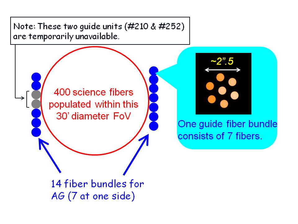
Auto guiding (AG) is performed by taking images of the guide fiber bundles (GFB) and calculating the centroids of GS. In total there are 14 GFB located at the edge of the field of view (FOV) as shown in Fig. 1a (NOTE: Two GFB are currently unavailable due to their less good positioning cababilities). The AG camera is a CCD camera with a long-pass filter (OG590, transparent at > 0.6 μm) in front of it. Observers therefore need to have GS bright in red optical bands and located near the edge of FOV. A guideline for GS brightness is R = 12 - 16 mag (this of course depends on seeing condition and sky transparency). Observers are highly recommneded to choose field center and PA to maximize the number of available guide stars: The more guide stars are available, the more stable AG operation is expected. Especially, the operation should be rubust against unexpected contamination of stars with large proper motions, double stars, those with large errors in astrometry, magnitude, etc. In addition, if all GS are bright, the exposure time for AG could be shortened. Then telescope pointing correction could be applied at a shorter interval and subsequently guding error could be smaller.
- Coodinate calibration stars (CCS)
These stars are used to align the telescope and instrument to the target field and acquire GS on GFB, by applying corrections to the telescope pointing and/or instrument rotator angle. This alignment (or field acquisition) process is necessary because:
- The typical pointing error of the telescope (≈ 4-5 arcsec) is larger than the FOV of GFB (≈ 2.5 arcsec in diameter), GS are not necessarily acquired by GFB after telescope pointing.
- If a rotational offset remains, it cannot be fully corrected by auto guiding, resulting in a significant amount of flux loss of science targets.
NOTE(1): The CCS near the center of FOV is also used for focusing operation: The same magnitude limit as other CCS (R = 12 - 15 mag) is applied. If there are CCS only at distances larger than 10 arcmin from the center of the FOV and one of those stars has to be used for focusing operation, the focus value derived could be less accurate due to the effect of curvature of focal plane.
NOTE(2): Observers may leave many CCS available in S2O files (see below for details about S2O file): Although the actual field acquisition is performed by using ∼ 5 CCS, if more CCS are available in an S2O file then the instrument control system picks up several from them considering the positions in the FoV.
- Run the spine allocation software
- The Spine-to-object (S2O) allocation software is still updated
from time to time for bug-fix and upgrade. The latest version has
been ready to try since Jun 30, 2011. However, due to the recent
incident of the telescope, unfortunately, the engineering
observations in July and August were both canceled, and we have not
been able to confirm yet if S2O files created by the latest version
work in actual observation.
Accordingly, we request S11B observers to download an older version (20101007 version) from the link below and prepare s2o files using it. In fact, there are several known issues on this version, but workarounds are available for most of them. S2O files created by this version have been working in observations.
- Spine-to-Object (S2O) allocation software (20101007 version) for Linux and Mac OS X (10.4 or higher). An HTML user manual is available in the "doc" directory. Several examples of catalogs are also available in the "examples" directory.
- Known issues on this 20101007 version
Note that there will be an engineering observation in Sep 2011, so the latest version of S2O software may be available for observers whose observations have been scheduled later in S11B.
- In S11B, HR as well as LR will be available on IRS1, while IRS2 will still be operated only in LR.
- Field center
- Position angle
- Observing wavelength
Due to the effects of atmospheric dispersion and chromatic aberration, the position of an object on the focal plane is slightly different as a function of wavelength. Observers therefore need to rightly input "observing wavelength" in the S2O software. Below listed is the guideline of observing wavelength for each observation mode:
Observing mode Observing wavelength Low resolution 1.3-1.4 μm High resolution J-short 1.0 μm J-long 1.20-1.25 μm H-short 1.50-1.55 μm H-long 1.65-1.70 μm - Observation date
- Maximal hour angle acceptable for observation
- Source list (priorities can be given to the science targets)
- RA & DEC offsets for beam switching (unless the observing method is Point & Stare - see below)
- Observing method
- Normal beam switching --- In this mode, the telescope is offset between "ON" and "OFF" positions, where the fibers look at objects (sky) at the "ON" ("OFF") position, respectively. Half of the observation time will be spent for sky exposure.
- Cross beam switching --- In this mode, two fibers are allocated to one object, and the telescope is offset between two positions so that either of the two fibers observes the object and the other observes sky. The advantages of this method are: (1) 100% of the time can be spent observing objects, and (2) at least in principle, sky subtraction is not affected by time variation of sky brightness. The disadvantage is that the maximal number of spines allocated to objects is 200. Since the geometrical constraint to spine allocation is strong, the actual number of allocated spines could be even smaller in reality.
- Point & stare --- There is no telescope offset in this mode. Instead, some fibers need to be placed on blank sky region and the average of the sky spectra is applied to other fibers for sky subtraction. For example, when most of the objects are relatively bright and the accuracy of sky subtraction is not extremely critical, this mode can be used.
- Maximizing the number of high priority targets with spines allocated
- Maximizing the number of guide stars located on the guide fiber bundles
- Minimizing spine tilts
- Avoiding spines to cross each other
- Save the output file(s) (*.s2o) and send it to the contact person(s) for FMOS open-use observation.
- Prepare an OPE file
- What is OPE file?
- How is it used?
- Template OPE file
Observation Procedure Execution (OPE) file contains a list of abstract commands to operate the telescope and instrument in actual observations. Like the other instuments on Subaru, observers using FMOS will also need to prepare an OPE file according to their plans of data acquisition during a night. Target information, observing method, exposure time, and so on will also need to be specified in this file.
In an actual observation, the content of an OPE file is displayed on the main telescope system control GUI. A support astronomer or telescope operator then selects the line for a certain command in it (with parameters in many cases) to execute when it is necessary. Observations proceed usually by repeating this for different commands.
Although an OPE file can be edited on the GUI during a night, to minimize overhead, it is important for observers to provide all the target information and prepare all the commands in OPE files that are used in their observations. On the other hand, since a command is manually picked up from an OPE file and is executed one by one, it is not extremely important to organize the commands exactly along the time sequence in an OPE file.
A template of OPE file for FMOS observation is available here:
Observers will need to download the text version of template and edit it to make one for your observation. Please refer to the PDF version as a brief manual. Then it needs to be sent to the support astronomer for FMOS open-use observations (Kentaro Aoki ).
).For clarity, please name your OPE file following the format "PROPOSALID_PILASTNAME.ope". For example, if your proposal ID is S10A-000 by PI: Tamura, then the name of an OPE file would be "s10a_000_tamura.ope". Again the OPE file name needs to be CASE-INSENSITIVE: Except for the extension (".ope", which has to be lower case), either upper-case or lower-case characters can be used for the file name but please do not mix them.
Observers first need to make a list of coordinates for science targets, guide stars, and coordinate calibration stars (see below for details of the latter two). All the candidates can be included in the list at this stage, since target selection for an optimal spine allocation will be performed by a software (see the next section). To ensure the accurate spine allocation and subsequently minimize flux loss from the fibers, observers need to be careful about the following things:
 |
 |
|||
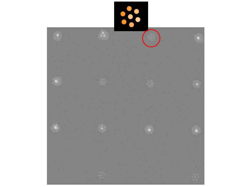
| Fig. 1a - A sketch of the guide fiber bundles. Note that two guide fiber bundles are unavailable due to their less good positioning cababilities. | Fig. 1b - A collection of the images of 14 guide fiber bundles during an actual auto guiding. 9 guide stars are clearly visible around the center of each bundle. |
|
!! Important notes for S11B observers !!
|
Observers will need to prepare and provide the information as below using this S2O software:
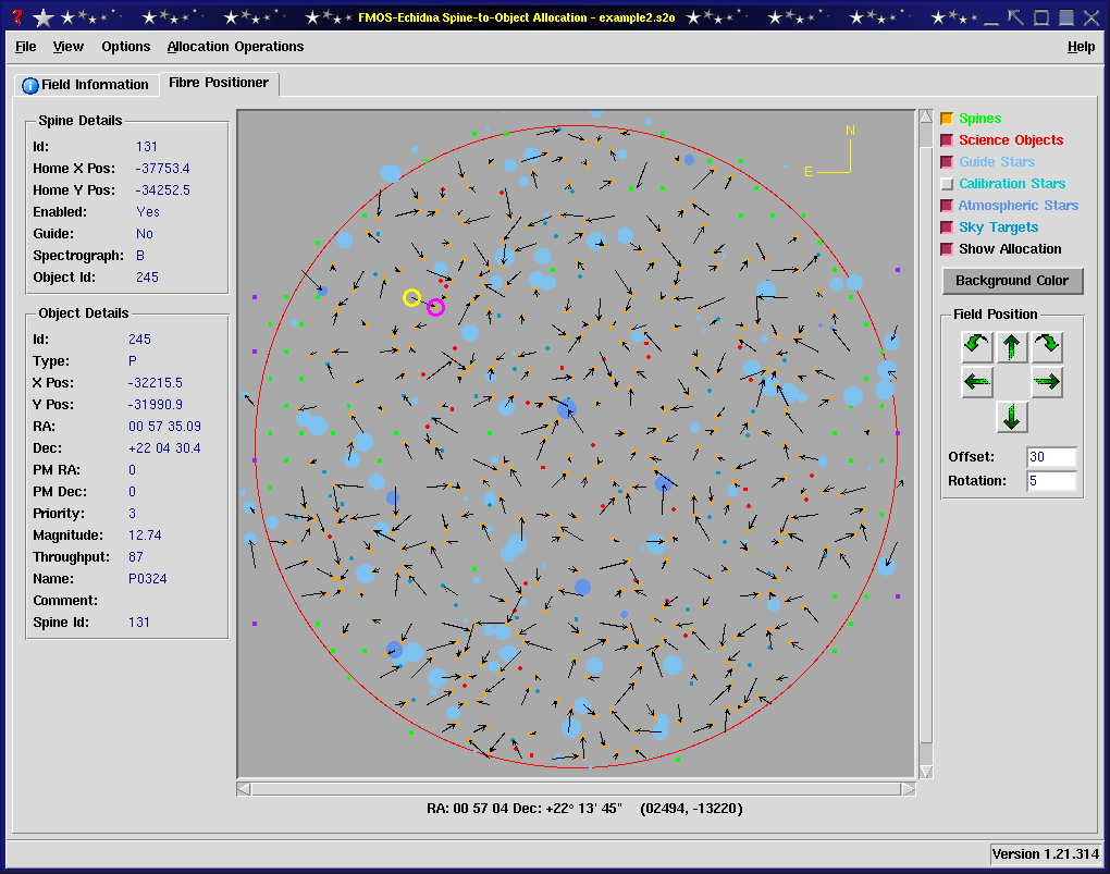
Fig. 2 - A snapshot of the spine allocation software. The arrows show the spines allocated to science targets or guide stars.
The spine allocation software produces an output file (*.s2o). According to the information in this S2O file, the Echidna Instrument Control Software (ICS) will configure the positions of the science fibers and guide fiber bundles for actual observations.
To finalize the spine allocation, please refer to the items in this check list and check if everything is considered properly.
Observers should send the final version of S2O files to support
astronomer(s) for FMOS open-use observations
(Kentaro Aoki ). If you observe more
than one spine allocations/target fields, please send all the
corresponding S2O files.
For clarity and maintenance purpose, please name your S2O files following the format "PROPOSALID_PILASTNAME_ANYCOMMENT_OBS.s2o". In the "ANYCOMMENT" part, observers can choose a useful phrase to classify the file (e.g. name of target field). "OBS" should be replaced with one of "nbs", "cbs", or "pas" depending on the selected observing method: Normal Beam Switching, Cross Beam Switching, or Point & Stare, respectively (see above in this section for the details of the observing methods). For example, if your proposal ID is S10A-000 by PI: Tamura and you observe a target field named "somewhere" by cross beam swiching, then please name the S2O file as "s10a_000_tamura_somewhere_cbs.s2o".
NOTE: S2O file name needs to be CASE-INSENSITIVE. Although it is OK to write an S2O file name using either all upper cases or all lower cases, please DO NOT mix them. For example, tamura.s2o and TAMURA.S2O are recognized as the same file by the Echidna ICS.
Observation procedure
- Pointing the telescope, rotating the instrument, configuring spines, & checking the focus
- Target field acquisition by making corrections to telescope pointing and instrument rotator angle
- Start auto guiding, and take exposures
- Operations of IRS1 and IRS2 are independent. For example, observers can set up IRS1 for LR and IRS2 for HR if wanted. Also, as long as the telescope stays at a certain position and the fiber configuration stays the same, exposures by IRS1 and IRS2 do not need to be synchronized: Duration of individual exposure and number of exposures can be chosen independently.
- As indicated in the "basic instrument parameters" page, currently the readout noise of the detector in the spectrographs is not very low. In a Correlated Double Sampling (CDS) readout, this noise will have to be fully included to every output frame. However, the noise level can be significantly reduced by exploiting non-destructive readouts (i.e. ramp sampling): Given an observer wants to take an 1800 sec exposure, the pixel count can be measured N=(1800/(minimum exposure time)) times in the process of exposure and the final frame can be obtained by a linear fit to the N data points. This is expected to reduce the readout noise by a factor of sqrt(N). Observers are therefore recommended to use this ramp sampling unless they need to repeat very short exposure.
- Since the rotator axis is slightly misaligned with the optical axis of the telescope main mirror, the pattern of field distortion on the focal plane rotates as the instrument rotates.
- Strength of differential atmospheric dispersion effect changes as the telescope elevation changes.
- Plate scale changes, e.g., when the truss temperature changes, and subsequently the distance between the telescope primary mirror and wide-field corrector in the PIR changes.
The typical overhead to complete 1. and 2. and get ready to start exposures is ~20 minutes, which is usually dominated by the spine configuration time. Spine configuration can start with slewing the telescope and rotating the instrument. The overhead will be longer when the telescope pointing is involved with a large amount of dome rotation and/or when the next target field is still at EL<30 degree: Since the spine configuration should be executed at a telescope elevation NO LOWER THAN 30 degree, the telescope elevation is temporarily raised to 40 degree to do a spine configuration.
Notes for operation:
Unfortunately, even if the instrument is rotated as necessary, the positions of objects on the focal plane gradually change as time goes by for several reasons as below:
Consequently, before flux loss from fibers starts being significant due to a large displacement between fiber and object positions, the spine positions need to be re-configured at a regular interval to keep observing the same objects with the same spine configuration. In the recent engineering observations, it has been confirmed that re-configuring the spine positions every 30 minutes enables the object flux to be reasonably constant. Each re-configuration process takes about 10 minutes. The typical observation efficiency in long integration is ~60% (i.e. the overhead is ~40%), while the efficiency gets lower for shorter integration because the contribution of initial configuration time (20 minutes) becomes more significant.
As of Feb 2011, we are still in the process of characterization and optimization and this frequency of re-configurations may be reduced in future as the instrument characteristics are better understood. However, the observers are strongly recommeneded to follow this sequence (i.e. executing the re-configuration process every 30 minutes) for long integration.
Data acquisition for flat fielding and calibration
- Flat fielding
- Wavelength calibration
- Telluric absorption correction and flux calibration
Dome-flat frames are taken in the evening and/or morning by closing the dome and using the dome-flat lamp. In doing this, the Echidna spines are configured to the same as for a scientific exposure. If observers have more than one target field/spine configuration to observe, then they would need to take the same number of sets of dome-flat frames with the spine configuration changed as appropriately.
A Th/Ar lamp is available in the buffle structure of the tertiary mirror pointing to the focal plane at the prime focus. Using this lamp, CAL frames are taken in the evening and/or morning (spine configuration at the time of this data acquisition should not matter for the accuracy of the calibration). A line list will be provided on this web site in the near future.
What has been usually done so far is to assign a few fibers to observe faint stars simultaneously with science targets. A guideline of the brightness of stars for this method is 15-18 mag (AB) in JH. The brighter limit of this range is set to minimize the effect of ghost features after the typical exposure time of an individual frame (i.e. 15 min), which tends to appear at a three-orders-of-magnitude (i.e. 7.5 mag) fainter level than the original brightness. The fainter limit is set to keep S/N of these stellar spectra high enough for calibration. The spectral types preferred are F, G, and K early dwarfs (A stars can be handled by the reduction package but are not recommeneded). Broad-band colors are expected to be useful to select them in advance, while it is also possible to estimate spectral type from observed spectrum, given the instrument throughput.
In theory, such correction/calibration is possible if one star is observed per spectrograph, but it is strongly recommended to observe a few to several stars possibley of different types so that the result of the correction/calibration can be cross-checked.
An alternative method is to observe a standard star in a different field before and/or after observing a science target field. Observers would need to prepare an S2O file for a standard star observation separately from those for science target field observations, where field center, CCS, & GS are necessary in the same way as science fields. This method would be recommended e.g. when a target field is at a low Galactic latitude and standard stars available there as well as science targets are highly affected by Galactic extinction.
Operation of high resolution mode
In the High Resolution mode (HR), the FMOS spectral coverage (0.9-1.8 μm) is divided into four pre-defined bands ("J-short", "J-long", "H-short" & "H-long") with a band width of ~0.25 μm, and one of them is observed at one exposure with a spectral resolution of ~5A. Please check this page for the basic parameters and this page for the sensitivity information.In S12A, HR as well as LR will be available on both IRS1 and IRS2. There will be a few restrictions to the HR operation as follows, and applicants/observers should keep them in mind about the use of HR:
- The FMOS spectral coverage (0.9-1.8 um) is divided into four bands in HR: J-short (0.90-1.16 μm), J-long (1.09-1.35 μm), H-short (1.40-1.66 μm) & H-long (1.54-1.80 μm), and one of them is covered by a single exposure. HR observation is carried out by using these pre-defined bands only. Note: More flexible operation may be possible in future semesters, but as of Aug 2011 more engineering works will be necessary to do so. Hence we decided to apply the restriction in S12A (i.e. the first semester of HR open-use) to minimize any technical risks.
- To minimize the risk of increasing additional overhead, observers need to keep the same setting of IRS1 & IRS2 from beginning to end of a night - i.e. No change is allowed in observation mode (e.g. LR → HR, HR → HR but a difference band) during a night.
- It would be acceptable to use IRS1 and IRS2 in different observation modes (e.g. LR in IRS1 and J-long in IRS2), while it is strongly recommended to use IRS1 and IRS2 in the same mode to accurately position Echidna spines/fibers: Due to the effects of atmospheric dispersion and chromatic aberration, the position of an object on the focal plane is slightly different as a function of wavelength, and the spine-to-object (s2o) allocation software cannot allocate spines according to different requests (e.g. observation wavelength) to spines for IRS1 and those for IRS2. This means, if one tried observation in J-long with IRS1 and in H-long with IRS2 and set observation wavelength for spine allocation to 1.3 μm, more light would tend to be lost at the fiber entrance for the H-long observation.